
ELISA Data Processing with Curve Expert and Operating Instructions
After completing ELISA sample assays and obtaining raw OD data, you enter the data‑analysis phase, where a set of practical questions arise: how should standard‑curve data be imported correctly? What are the standardized workflows for constructing and evaluating the fitting performance of a standard curve? How can concentrations of unknown samples be accurately calculated?
In ELISA experiments, standards and test samples are generally measured in 1‑2 replicate wells. First, calculate the mean absorbance for standards and each sample group. The deviation between individual well readings and their corresponding mean value should not exceed 20%. Subtract the mean OD value of blank wells from sample mean OD values to finish background correction, then build the standard curve based on corrected data.
ELISA quantification establishes a functional relationship between concentration and absorbance using reference standards. Select an appropriate model for curve fitting, assess goodness‑of‑fit, and back‑calculate analyte concentrations of unknown samples with the fitted equation. Standardized replicate‑well quality control, background subtraction, standard‑curve fitting and sample‑concentration calculation are core steps to convert high‑quality raw experimental data into reliable quantitative results.
This article uses Curve Expert software to demonstrate step‑by‑step procedures for data import, standard‑curve plotting, goodness‑of‑fit evaluation and concentration calculation for unknown samples.
1. Import ELISA Standard Data into the Software
1.1 Download and launch Curve Expert, then open a new worksheet.
1.2 Enter OD values and corresponding concentrations of standard substances, or directly paste data copied from Excel.
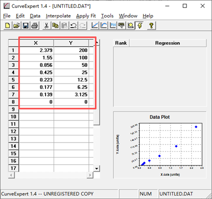
1.3 Click the CurveFinder button to pop up the dialogue box shown below. Click [OK]; the software will start curve plotting and automatically return the curve with the best fitting performance upon completion.
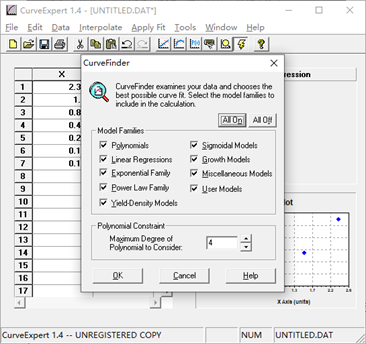
2. Select a Suitable Fitting Model
After curve‑fitting analysis, inspect fitting outputs of different regression models and select the one that best matches the response trend of standard samples.
Statistical parameters such as correlation coefficients can be used to evaluate fitting quality. However, do not treat “r value approaching 1” as the sole criterion for model selection.
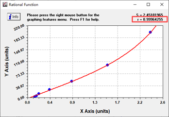
3. Calculate Sample Concentrations from the Standard Curve
Once a valid standard curve is generated, use the software to determine the concentration corresponding to the OD value of each unknown sample.
3.1 Perform Calculations within Curve Expert
Right‑click blank space in the dialogue window, select “Analyze”, choose calculate Y from X, input the OD reading and click “Calculate” to obtain the corresponding protein concentration. If specimens were diluted N‑fold before testing, multiply the calculated value by N for the true protein concentration.
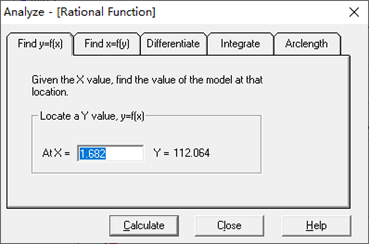
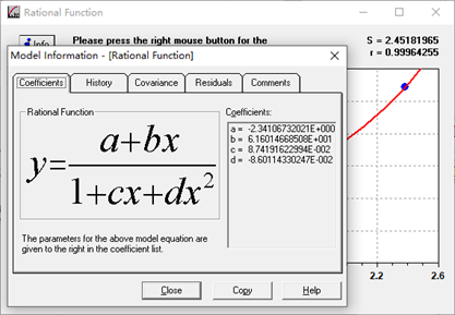
3.2 Access Curve Equation
Right‑click blank space in the dialogue window and select “Information” to view the curve equation. Click “Copy” and you may paste the equation wherever required.
Important Notes:
For reliable quantitative results, sample readings should ideally fall within the usable range of the standard curve. If samples were diluted prior to measurement, the dilution factor must be incorporated when computing final concentrations.